Let’s say you are in the middle of a salary negotiation, and you want to know whether you should be aggressive in your offering or conservative. One way to help with the decision is to make a decision tree. We’ll work with the following assumptions:
- You are at a job currently making $50k
- You have the choices between asking $60k (which will be accepted with probability 0.8) or $70k (which will be accepted with probability 0.2).
- You get one shot. If your asking price is rejected, you stay at your current job and continue to make $50k. (This is one of those simplifying assumptions that we might dispense with later.)
This simplification of reality can be represented with a decision tree:
I went ahead and put in the expected payoff for each of these decisions. Because the more conservative approach has a higher expected payoff, this model suggests that you should take the conservative approach.
One shortcoming clearly is that this decision tree only shows two decisions, but really you have a range of decisions; you are not stuck with $60k or $70k for asking price. You might go with $65k, or $62.5k, or something else. So what would be the optimal asking price?
Again, we look at expected payoff, which is asking price*probability(offer accepted) + $50k * probability(offer rejected). In this case, we need to model the probability that offer is accepted over the range of possible offers, not just the two points. The logistic model works very well for modeling probability, and that’s what I will use here to extend the two-point model. In fact, a logistic model with two parameters can be fit exactly to two points, and so that is what I will use here.
Here is my commented R code to implement this model:
my.offer <- function(x1=60,py.x1=.2,x2=70,py.x2=.8,ev.no=50,high=100,p.payoff=1) {
  # return the offer to maximize expected payoff
  # this assumes a game with one decision and one consequence
  # you give an offer, and it is taken or refused. If taken, you receive a salary of
  # (a function of) the offer. If refused, you stay at the old job and receive a
  # salary of ev.no (presumably a current salary, but set to 0 if you are
  # unemployed).
  # the probability of rejection is modeled with a logistic function defined by
  # two points (x1,py.x1) and (x2,py.x2)
  # for example, if you expected a 20% rej. prob. with an offer of 140k, then
  # x1,py.x1 = 140,.2. Similarly with x2,py.x2
  # the expected payoff is modeled as offer*P(Yes|offer) + ev.no*P(No|offer),
  # perhaps with  modifications to account for benefits, negotiation, etc. This
  # is defined in payoff function below.
  # finally, high is defined as anything above what you would be expecting to offer
  # and is used to create the plot limits and set the bounds in the optimization
  # routine.   # model the probability of no given salary offer
  # here we have a logistic function defined by (x1,py.x1) and (x2,py.x2)
  # note that qlogis is the inverse logit function
  # also, matrices in R are defined in column-major form, not row-major form like
  # FORTRAN, so we have to use 1,1,x1,x2 rather than 1,x1,1,x2
  theta <- solve(matrix(c(1,1,x1,x2),nc=2),matrix(qlogis(c(py.x1,py.x2)),nc=1))   # for plot of probability function
  xseq <- seq(ev.no,high,length=100)
  yseq1 <- 1/(1+exp(-theta[1]-theta[2]*xseq))   # model the expected payoff of an offer
  # model negotiations, benefits, and other things here
  # (a simple way to model benefits though is just to change ev.no)
  payoff <- function(x) {
    tmp <- exp(-theta[1]-theta[2]*x)
    return( (ev.no + ifelse(ev.no>x*p.payoff,ev.no,x*p.payoff)*tmp)/(1+tmp) )
  }     yseq <- payoff(xseq)   # plots
  par(mfrow=c(1,2))
  plot(xseq,yseq1,type='l',xlab='Offer',ylab='P(No|X)')
  plot(xseq,yseq,type='l',xlab='Offer',ylab='Expected salary')   # no sense in even discussing the matter if offer < ev.no
  return(optimize(payoff,interval=c(ev.no,high),maximum=TRUE))
}
Created by Pretty R at inside-R.org
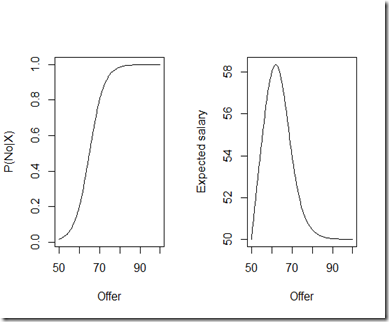
And here are the graphs and result:
> my.offer()
$maximum
[1] 61.96761

$objective
[1] 58.36087
So this model suggests that the optimum offer is close to $62k, with an expected payoff of around $58k. As a side effect, a couple of graphs are produced: giving the probability of rejection as a function of the asking price, and the expected salary (payoff) as a function of asking price.
So a few comments are in order:
- The value in this model is in varying the inputs and seeing how that affects the optimum asking price.
- The function I provided is slightly more complicated than what I presented in this post. You can model things like negotiation (i.e. you may end up at a little less than your asking price if you are not turned down right away), differences in benefits, and so forth. Once you have a simple and reliable baseline model with which to work, you can easily modify it to account for other factors.
- Like all models, this is an oversimplification of the salary negotiation process, but a useful oversimplification. There are cases where you want to be more aggressive in your asking, and this model can point those out.
- I commented the code profusely, but the side effects are probably not the best programming practice. However, this really is a toy model, so feel free to rip off the code.
- This model of course extends to other areas where you have a continuous range of choices with payoffs and/or penalties.
- If you are able to gather data on the probability of rejection based on offer, so much the better. You can then, instead of fitting an exact probability model, perform a logistic regression and use that as the basis of the expected payoff calculation.

